Simulating gambling tactics
Table of Contents
This is a story about one time when I was and I stumbled upon a new domain of interest. This interest was related to gambling and it occured when a friend of mine told me of a “foolproof” betting strategy for the game of roulette.
The gambling strategy #
For any games where there is a near 50% chance of winning and where winning doubles your money and losing loses all your money you do this: First bet $1, if you lose this bet instead of betting $1, on the next turn you bet $2 (double the previous bet), if you lose again, bet $4, then $8 etc. If you win however, you restart the betting number and bet $1 again. So the tactic is basically double-down each time you lose. In the above scenario, if you lose the first bet, you are down $1, if you lose the second bet you are then down $3 ($2 + $1), if you lose the next bet you are down $7 ($4 + $2 + $1) etc. Whenever you win, assuming you eventually win, you will be net positive. For example if you were down $3 and you then bet $4, you would then be up $1 in total. Below there is a table to illustrate this:
| Current Bet | Net Money | If you win this bet (but lost all previous ones) |
|---|---|---|
| 1 | 0 | 1 |
| 2 | -1 | 1 |
| 4 | -3 | 1 |
| 8 | -7 | 1 |
| 16 | -15 | 1 |
Now although $1 is a small amount to win, this $1 is an arbitrary number, it could me multiples of 1000 (in this case multiply everything by 1000) and therefore each time you win, you would win $1000. The point is, supposing you have enough money you could hypothetically keep winning and the only way to lose is to lose X amount of times in a row so you don’t have any money.
I have embarked on a journey to see whether this theory holds true using some basic coding, data science and maths.
Writing some code #
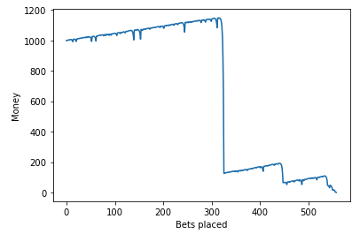
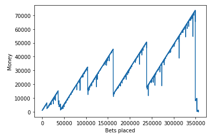
First I created a simulation in python to simulate an agent (the gambler) betting their money and using the strategy (using different parameters that I will describe below) to see what would happen. I graphed the first couple of games to get a general feel to what was happening:
Some maths #
It seemed that my agent always somehow ran out of money and the money always eventually goes to zero. After doing a tiny bit of research I found a few things. First, this tactic is a popular roulette tactic called the “Martingale tactic” where you double the bet each time you lose. Second, there were two interesting mathematical theories that were closely related to what I was experimenting on. Gambler’s ruin and random walk
Gambler’s ruin is a statistical concept that describes the probability of winning when 2 people are betting against each other. The probability is directly proportional to the amount of money player 1 has in relation to player 2. Assuming that player 1 has finite wealth and player 2 has basically infinite wealth (the casino), eventually player 1 will go broke. This can be modeled by a random walk, a concept that describes the path of randomly occuring events (in our case, winning and losing the bet). If we imagine the y-axis is the amount of money we have and the x-axis is each new bet, the random walk will look something like this (courtesy of Vladimir Ilievski. Ignore the axis labels)
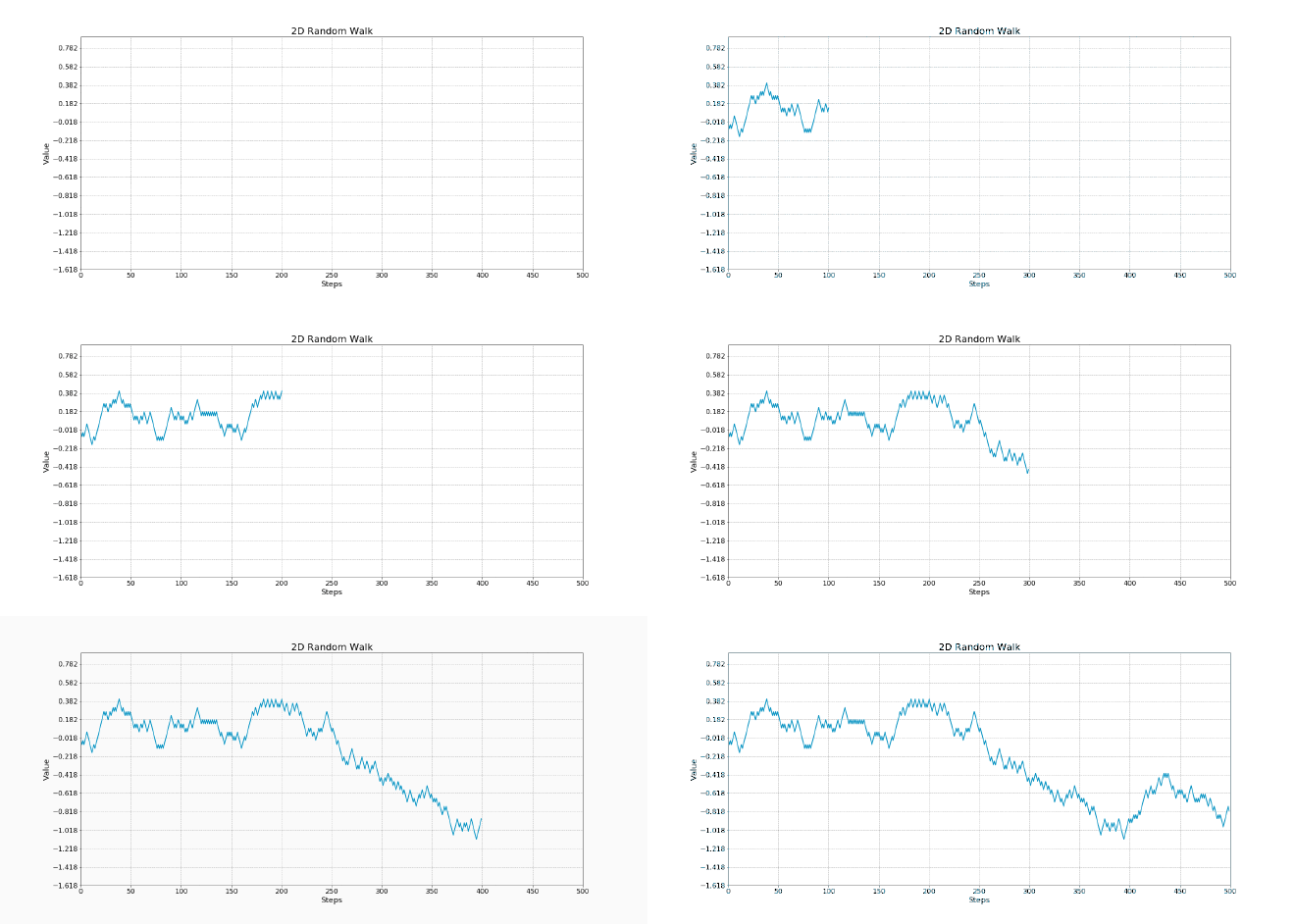
No matter how lucky a person is, eventually the random walk will lead to the player having no money.
Understanding the maths a bit more, the agent starts with M money, this means they can lose \(log_2(M+1)\) times in a row before they go bankrupt, we will call this \(Z\). e.g If the agent starts with $1023, this means they would lose all their money if they lost
$$Z=log_2(M+1)=log_2(1024)=10$$
times in a row
(This is because after losing once, you lose $1, then $2, $4, $8, $16, $32, $64, $128, $256, $512. Adding all these up, this means you will have lost $1023. Meaning it takes 10 losses in a row to go bankrupt)
So I hit a dead end. You can’t use the Martingale tactic to make millions of dollars from casinos. Or can you???
I wanted to keep exploring this tactic by changing some of the parameters. The parameters were starting money M, what you do to the bet when the agent loses \(X\) (for example when doing double or nothing, \(X=2\)), and the win percentage.
Questions arose including: what would happen if I increase X, would it lead to more winnings, more volatile games? If I increase my win percentage, is their a way to guarantee increasing your money? How does increasing \(M\) affect my final winnings?
Testing different values of \(X\) #
Using my program, I attempted to change the value for \(X\), making it triple or nothing, quadruple or nothing etc. Unfortunately, from this, nothing of value came. It did not lead to an increase of money, however when testing its affect against the number of bets placed before going bankrupt, this was the result
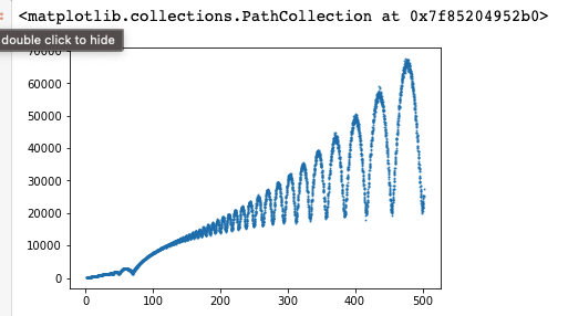
Where the x axis represents the x value, the y axis represents the number of bets placed before losing (the start money was 5000). Interesting pattern, but nothing to do with increasing winnings.
Testing different values of \(M\) #
I created a function which tested different \(M\) values and their likelihood of doubling their money. For 15 different \(X\) values, I created the corresponding \(M\) value (\(2^x\)) (i.e for 2,4,8,16,…, 16384,32768) I then tested for each M, the probability that it would double their money. Looking at the experimental data, my hypothesis was wrong and in fact the amount of starting money you have will not impact yout chances of doubling your money.
Modelling the probability #
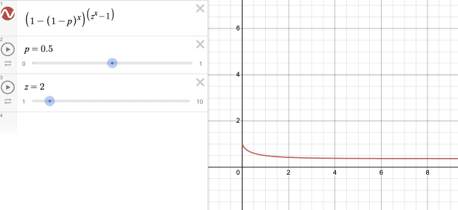
I was curious how all these parameters affect the probability of winning, this is what I came up with. It doesn’t line up completely with experimental data though.
$$P = (1-(1-p)^x)^{z^x-1}$$
This equation is the full equation describing this phenomenon
\(P\) is the probability of \(z\) ing your money (if \(z\) is 2, doubling your money)
\(p\) is the probability of winning a single game
\(X\) is the amount of games you can lose in a row before going bankrupt
\(z\) is what the agent does after losing (if \(z\) is 2, double or nothing, 3 is triple or nothing)
I first broke this problem down into its individual components. First, what is the probability of winning/losing a single game. For simplicity, we will have odds of 50/50 and so the probability of winning and losing is 0.50. Now, what is the probability of losing \(x\) games in a row. The probability will be \(0.5^x\). Therefore if you want the probability of not losing \(x\) games in a row, it will be \( 1-0.5^x \). Now lets say you want to do this \(z\) times. To do this successfully \(z\) times, it will be \(1-0.5^x \times 1-0.5^x \), \(z\) times. Therefore it will be \((1-0.5^x)^z\) where \(z\) is the number of times you want to win. Now, the formula below represents the full equation with all the variables. Plotting this out gives this graph.
Some realisations #
No matter what I did, it seems if the odds are 50/50, there is no way to have an edge through leveraging your money or using a certain tactic. These are the rules of probability and it is not possible to “beat luck” and have a systematic method to improve your chances.
More research led me to Ed Thorpe’s article about the Martingale Tactic (https://www.edwardothorp.com/wp-content/uploads/2016/11/SystemsForRoulette_l.pdf) as well as a good book called The Theory of Gambling and Statistics (https://au1lib.org/book/702712/119692). In Chapter 3: The Basic Theorems, Epstein dispells the myth of the Maringale tactic working and reiterates what I have written here.
Conclusion #
As I was nearing the end of my research on this topic, I was reading a book about gambling and in it, it said
If a gambler risks a finite capital over a large number of plays in a game with constant single-trial probabilities of winning, losing, and tying, then any and all betting systems lead ultimately to the same mathematical expectation of gain per unit amount wagered.
There is no way to beat a system where the “odds” are not in your favour. Although you may be able to win a few times, as you keep attempting the tactic, your chances of winning money will decrease as time goes on.
Give up. Don’t go to the casino.
Appendix #
Here’s a link to the code in python and in c++ if you want to play around
https://github.com/josephf123/gamblingSimulator
A strange graph relating X value and number of bets placed before going bankrupt. I wonder why it forms this shape? Also, this was actually when the code had a bug in it and when winning a bet, the betting amount doesn’t reset.
Why is it when I do experimental data on what the probability of doubling your money asymptotically approaches, it goes to 1/\(e\) in theory but in practice it is just 1/2?
Why the model is not exact:
- it is not accounting for losing \(x\)/2 in a row and then another \(x\)/2 in a row?
- How many ways can you lose
- How many ways can you win
- Recursive formula? There are infinite ways to get back to the same spot.
For the function:
$$P = (1-(1-p)^x)^{z^x-1}$$

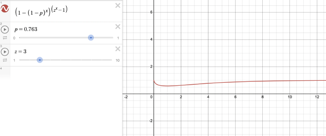
Depending on the parameters, the graph will either have an asymptote at 1, 0 or 1/\(e\).
It seems there is a pattern for when the graph has an asymptote at 1/\(e\).
$$ p = 1 - \frac{1}{z} $$
If \(p > 1 - 1/z \), the odds will converge to 100% and if \(p < 1 - 1/z \) the odds will go down to 0%.